Something as shown below:
There is a dual functionality to this – you can select a country’s name from the drop-down list, or you can manually enter the data in the search box, and it will show you all the matching records. For example, when you type “I” it gives you all the country names with the alphabet I in it. Download Example File and Follow Along Watch Video – Creating a Dynamic Excel Filter Search Box
Creating a Dynamic Excel Filter Search Box
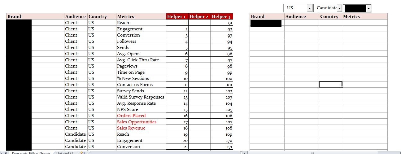
This Dynamic Excel filter can be created in 3 steps: Here is how the raw data looks:
USEFUL TIP: It is almost always a good idea to convert your data into an Excel Table. You can do this by selecting any cell in the dataset and using the keyboard shortcut Control + T.
Step 1 – Getting a unique list of items
NOTE: If you use ‘Remove Duplicates’ method and you expand your data to add more records and new countries, you will have to repeat this step again. Alternately, you can also you a formula to make this process dynamic.
Step 2 – Creating The Dynamic Excel Filter Search Box
For this technique to work, we would need to create a ‘Search Box’ and link it to a cell. We can use the Combo Box in Excel to create this search box filter. This way, whenever you enter anything in the Combo Box, it would also be reflected in a cell in real-time (as shown below).
Here are the steps to do this:
Step 3 – Setting the Data
Finally, we link everything by helper columns. I use three helper columns here to filter the data. Helper Column 1: Enter the serial number for all the records (20 in this case). You can use ROWS() formula to do this. Helper Column 2: In helper column 2, we check whether the text entered in the search box matches the text in the cells in the country column. This can be done using a combination of IF, ISNUMBER and SEARCH functions. Here is the formula: This formula will search for the content in the search box (which is linked to cell K2) in the cell that has the country name. If there is a match, this formula returns the row number, else it returns a blank. For example, if the Combo Box has the value ‘US’, all the records with country as ‘US’ would have the row number, and rest all would be blank (“”) Helper Column 3: In helper column 3, we need to get all the row numbers from Helper Column 2 stacked together. To do this, we can use a combination if IFERROR and SMALL formulas. Here is the formula: This formula stacks all the matching row numbers together. For example, if the Combo Box has the value US, all the row numbers with ‘US’ in it get stacked together. Now when we have the row numbers stacked together, we just need to extract the data in these row number. This can be done easily using the index formula (insert this formula in where you want to extract the data. Copy it in the top-left cell where you want the data extracted, and then drag it down and to the right). This formula has 2 parts: INDEX – This extracts the data based on the row number. IFERROR – This returns blank when there is no data. Here is a snapshot of what you finally get: The Combo Box is a drop down as well as a search box. You can hide the original data and helper columns to show only the filtered records. You can also have the raw data and helper columns in some other sheet and create this dynamic excel filter in another worksheet. Download the Dynamic Excel Filter Example File Get Creative! Try Some Variations You can try and customize it to your requirements. You may want to create multiple excel filters instead of one. For example, you may want to filter records where Sales Rep is Mike and Country is Japan. This can be done exactly following the same steps with some modification in the formula in helper columns. Another variation could be to filter data that starts with the characters that you enter in the combo Box. For example, when you enter ‘I’, you may want to extract countries starting with I (as compared with the current construct where it would also give you Singapore and Philippines as it contains the alphabet I). As always, most of my articles are inspired by the questions/responses of my readers. I would love to get your feedback and learn from you. Leave your thoughts in the comments section. Note: In case you’re using Office 365, you can use the FILTER function to quickly filter the data as you type. It’s easier than the method shown in this tutorial.
Highlight Matching Data Using Conditional Formatting – Dynamic Search. Create a Search Suggestion Drop Down List in Excel. Using Advanced Filter in Excel. How to Extract a Substring in Excel (Using TEXT Formulas). Creating a Drop Down Filter to Extract Data Based on Selection. How to Filter Cells with Bold Font Formatting in Excel. Highlight Rows Based on a Cell Value in Excel.
what if i want to filter only unique record only? lets say in my data against the country japan “Product 7” is coming for 7 times but i want to filter it only one time . is it possible? For example if you want to see product category from both India AND China how do you change the equation? In this case we are trying to separate group of country and applying filter on them. Example I filter for India, it bring up 4 result and then I want to input data to the results. More like i’m filtering the actual entire row of the result? You response will be greatly appreciated. I’ve found your video extremely useful, but like a lot of others I’m struggling to apply your formula to multiple searches/filters/conditions. I’ve seen you’ve shared a dropbox link for this solution but they have expired. Is it possible to please create another link or to comment in an example of this formula – this would be much appriciated. Many thanks, Jack It really helped me do the search bar and it works fine, however, my data is huge and it takes lot of time to get the output and it keeps calculating. Kindly suggest on the concern. Can anyone help?? I hope that makes sense… I would love to know will I do the above statement. and btw thankyou for the video it really helo me a lot. the only thing that i need to do is the statment above. I hope you will answer this please I have different sheet each one of them have the same think just different company name. i want to have as in this exemple but result in an other sheet and also the data coming from different sheet thanks I need, please your help if you can. I want to know I want to create this filter first with more than 15 worksheets and each one having the same column and rows information. I want to create a comparison tool, as if, I enter for example item number or name will give me a grill with what I need in a unique worksheet as an output. Here is what I have : 1- 15 worksheets: each worksheet, it’s for a specific company, each sheet has the same thing: ex: item name, prices, capacity, our prices, margin, etc.. 2- I want to make a search ( as you did in the box you create ) when I search for example by name: *** My result expected: will give a table with the less price first and which company is associated with. 3- is it possible to do with excel, if not can you guide me please, which program I can need to use is it a database +VB or what exactly, please. Thanks a lot. I have successfully completed this; however, one of my columns with information the populates contains hyperlinks to documents on the computer. Right now these hyperlinks are only showing up as text. I would like the link to be retained when it appears in the search results, can you help with this? how can i improve this? email – varunsharma16@gmail.com Plz help me with sample file https://uploads.disquscdn.com/images/19ca56064e7652e5ae9209a5241c817f0644dc910843e1b1839187be278cae47.jpg I’ve just discovered a pretty good video where the search filter works dynamicaly by hiding the rows. Looks very nice and useful. Moreover, there is a download link below the video, so you can try it immediately. https://www.youtube.com/watch?v=iZ933-tU6Yw Maybe you will find there some new ideas.. If I have dates in mm/dd/year (or some equivalent) how can I use the dynamic filter to search by month or year whilst keeping the date format? Unfortunately even if the dates are formated to say the respective month it only searches in based off of what is in the formula box. I look forward to your response. Simply put this formula in F4 and copy for all the cells in that column. If I copy the formula over and add the sheet name before the cell I can see all the current values, but it doesn’t appear to be dynamic and update like the information does on the original sheet. any help is appreciated. This is a brilliant method for making a searchable staff telephone list. However, some of my cells in the range are blank, where there is either no extension or mobile, and they are showing in the search result table as 0. I have tried, without success, to add an if statement to weed these out and show them as blank cells. Is there a way to do this without causing the formula =IFERROR(INDEX($B$4:$D$23,$G4,COLUMNS($I$3:I3)),””) to throw up an error? Thanks for sharing! I am currently putting the dynamic filter and its data on a different worksheet. May I know if it is possible to also have a filter option to display “All the data”. If I would like to have the option to choose “All Countries” from your example, how would I be able to do it? Now when the combo box is empty, it will show no results I’m trying to do a version of this where the data is output to a second sheet (saves me from hiding & unhiding cells all the time). I’ve managed to output the data to a sheet named UI (user interface) but now the search filter isn’t working. It’s probably something to do with how I’ve written the Formula’s, but I can’t figure it out. I’ve attached screenshots showing the sheets and the formula’s being used. Any help would be much appreciated! Cheers, Jen I guess it has something to do with The helper 2 column “=IF(ISNUMBER(SEARCH($K$2,D4)),E4,””)” Could you please help me to search the result of the exact value? Thank you so much ! Only issue I encountered is after selecting the item from the Combo list, sometimes the selection just disappears – i.e. the combolist seems to just clear itself. Not sure what is going on there. Do you have any idea what could be causing this please? thank you in adance p.s. more about INDEX MATCH benefits: http://www.mbaexcel.com/excel/why-index-match-is-better-than-vlookup/ Thank you so much for uploading this video. Is there any way to show the search result blank if there is no data in the combobox ? Paste this formula in F4 and drag it down. Regarding the variations: I’m wondering if it’s possible to have more than two conditions/filters? I can’t seem to figure out the correct formula. Thanks! I’ve downloaded that version and applied the formula to my spreadsheet. It works perfectly for two conditions, but I can’t figure it out for more than two. Is this possible? Sorry if this isn’t clear! You need to modify the formula in second helper column to check for all 3 conditions You would need to club the 2 to get dynamic filter that retain hyperlinks Your example is too good but I don’t want to use “INDEX” formula. Please help me out. You wrote this “You can try and customize it to your requirements. You may want to create 2 filter instead of one. For example, you may want to filter records where Sales Rep is Mike and Country is Japan. This can be done exactly following the same steps with some modification in the formula in helper columns.” Could you please tell me what changes to make in helper columns to make 2 filters work? Thanks a lot! Kindly let me know. Best Regards, Karthik I have added another filter and changed the formula in the helper columns Sumit, Could you please tell me how to use 2 filters, i.e. what changes to make in the helper columns? Thanks Amal =IF(AND(G3″”,G4=””),SUM($G$4:G4),IFERROR(INDEX($B$4:$D$23,$G4,COLUMNS($I$3:J3)),””)) I have made it based on the data set I have provided in the download file (assuming Column C has numbers) {=IFERROR(INDEX($B$2:$D$21,SMALL(IF(ISNUMBER(SEARCH($U$1,$D$2:$D$21)),ROW($D$2:$D$21)-1,””),ROW()-4),COLUMNS($L$4:L4)),””)} I know it was a long time ago, but if you could possibly reply with the rest of the formula i would really appreciate it! Isaac
